The unknown is a small nitrogen-containing natural product. Use the supplied evidence to propose a constitution before consulting the reviewed solution. Record what each experiment shows separately from what you think it means.
Learning goals
- Separate observation, interpretation, and confidence.
- Trace proton spin systems with COSY.
- Connect attached proton and carbon environments with edited HSQC.
- Test sequence and ring closure with HMBC.
- Compare the 400 and 600 MHz proton spectra without assuming that field strength is the only experimental difference.
Experimental context
Experiments 31–35 form one primary acquisition series in DMSO-d6 at approximately 298 K. Experiment 30 is an earlier proton acquisition at approximately 300 K and must be treated as a comparison rather than part of the same session. Proton chemical-shift scales were verified against the residual DMSO-d₆ resonance at 2.50 ppm (Cambridge Isotope Laboratories NMR Solvent Data Chart). The ¹³C axis currently reads the residual DMSO-d₆ septet near 40.0 ppm rather than the chart value of 39.51 ppm, so treat absolute ¹³C readings as provisional until the data are re-referenced.
| Stage | Experiment | What to establish |
|---|---|---|
| 1 | 1H NMR, 600 MHz | Count signal regions, inspect integrals and multiplicity, and identify exchangeable or overlapped signals. |
| 2 | J-modulated 13C NMR | Estimate the number and classes of carbon environments, including carbonyls. |
| 3 | COSY | Build independent proton spin systems before naming fragments. |
| 4 | Edited HSQC | Attach proton signals to carbon environments and distinguish phase classes supported by the experiment. |
| 5 | HMBC | Test how the spin systems connect and whether the carbonyl evidence supports cyclization. |
| 6 | 400 MHz comparison | Note changes in dispersion and apparent second-order behavior. |
Stage 1: Survey the proton spectrum
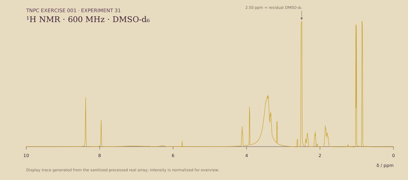
Figure 1. Processed 1H NMR overview for Experiment 31 (600 MHz, DMSO-d6). Intensity is normalized for display. The arrow marks the residual DMSO-d₆ resonance at 2.50 ppm, the chemical-shift reference (Cambridge Isotope Laboratories NMR Solvent Data Chart). Inspect the interactive data or download package before measuring shifts or integrals.
Create an observation table before assigning any atom labels. Which regions appear methyl-like, methylene-like, methine-like, or exchangeable? Which signals require the two-dimensional data before they can be separated confidently?
Stage 2: Account for the carbon environments
Use the J-modulated spectrum itself rather than relying on an automated peak list. How many carbonyl environments are visible? Which signals have phase behavior consistent with protonated versus non-protonated carbon classes?
Stage 3: Build spin systems with COSY
Trace each continuous coupling network. Keep separate networks separate until another experiment provides a connection. Mark ambiguous cross-peaks and test whether they survive a sensible contour-level change.
Stage 4: Connect protons and carbons with edited HSQC
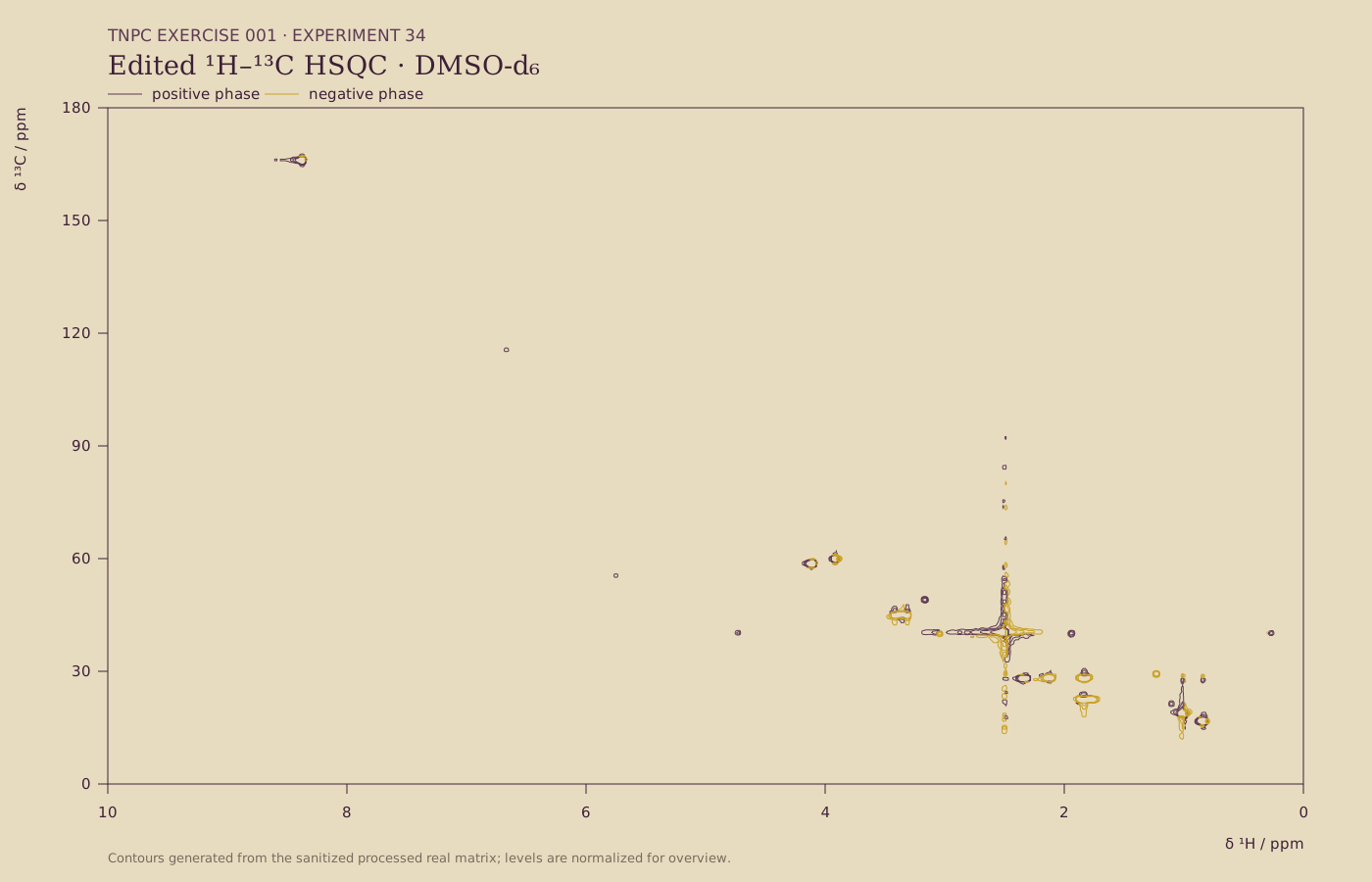
Figure 2. Edited 1H-13C HSQC overview for Experiment 34 (DMSO-d6). Green and orange contours show opposite phases. Contour levels are normalized for overview rather than quantitative comparison.
Transfer each resolved proton signal to its directly attached carbon. Preserve diastereotopic proton observations rather than compressing them into one value prematurely.
Stage 5: Test sequence and ring closure with HMBC
Focus on long-range correlations to the carbonyl regions. For each proposed connection, write down the observed cross-peak, the structural claim it supports, and at least one alternative it helps exclude.
Stage 6: Compare 400 and 600 MHz
Align the proton spectra by chemical shift. Which regions become easier to interpret at 600 MHz? Which differences may instead reflect separate acquisition sessions, processing, concentration, or temperature?
Submit your proposal
Prepare a structure proposal, a complete assignment table, and a short evidence chain. Clearly label any inference that depends on an absent, weak, or overlapped cross-peak.
Data downloads
The interactive viewer uses the sanitized processed-data package. For reproducibility, download the complete sanitized raw and processed archive (ZIP, 72.8 MiB) and its SHA-256 checksums. The source workstation folders remain unchanged and are not published directly.
Solution status
The structural reveal and reviewed assignment table are intentionally withheld while scientific review is in progress. Publishing the prompt first lets readers work from the evidence without receiving an unreviewed answer.